The aggregate impact of AI on Norwegian employment
Exposure, the wage it travels with, and their interaction — to 2026Q1
The question
Exposure scores say what AI could touch. They do not say what happened to jobs. This page asks the aggregate question on Norwegian register-style data: once general-purpose AI arrived, did the most-exposed occupations — and especially the well-paid, exposed ones, where the economics says displacement should bite first — lose employment?
Data & method
Panel. Quarterly STYRK-08 occupational employment and monthly earnings, 2016Q1–2026Q1, from Statistics Norway (SSB tables 12542 and 11418); AI exposure from Eloundou et al. (2024).
The regression. One observation per occupation. The outcome is the Yagan (2019) percent change in employment relative to its pre-ChatGPT average, \[y_o = 100\,\frac{E_{o,\,2026Q1} - \bar E^{\text{pre}}_o}{\bar E^{\text{pre}}_o}, \qquad \bar E^{\text{pre}}_o = \text{mean employment over quarters } \le 2022Q3,\] a level-robust alternative to a log difference (it does not blow up when the base quarter is small or noisy). We build it up in three nested steps, each regressor standardised (so coefficients are per 1 SD, in percentage points of employment), with heteroskedasticity-robust SEs:
- \(y_o = \alpha + \beta_1\,\mathrm{Exp}_o + \varepsilon_o\) — the naive exposure regression.
- add the pre-ChatGPT average log wage \(\ln \bar w^{\text{pre}}_o\) (mean monthly wage over 2016Q1–2022Q3) as a control — pre-determined, so it is not contaminated by the post period.
- add the interaction \(\mathrm{Exp}_o \times \ln \bar w^{\text{pre}}_o\).
Why this order. Exposure and pay are correlated (high-exposure office work is well paid: corr ≈ 0.55). So a raw exposure coefficient is partly just wage. Putting wage in as a control lets OLS net that out; the interaction then asks the sharp comparative-advantage question — does exposure cost more jobs precisely where pay is high? (prediction \(\beta_3<0\)). Because all three are entered together, \(\beta_3\) is the genuine, partialled interaction — there is no collinearity sleight of hand.
From one number to a path. The cross-section is a single long difference, so we also run the event-study (diff-in-diff) version: every coefficient gets a time subscript, estimated jointly with occupation and quarter fixed effects (ref. = 2022Q3, SE clustered by occupation), \[y_{o,t}=\alpha_o+\tau_t+\sum_{k}\big(\beta_{1,k}\,\mathrm{Exp}_o+\beta_{2,k}\ln\bar w_o +\beta_{3,k}\,\mathrm{Exp}_o\times\ln\bar w_o\big)\mathbf 1[t{=}k]+\varepsilon_{o,t}.\] We show it twice, exactly as in the deck: naive (\(\beta_{1,k}\) alone — what people usually estimate) and joint (all three entered simultaneously, so \(\beta_{1,k}\) is exposure net of wage and \(\beta_{3,k}\) is the genuine heterogeneity-by-wage interaction).
Robustness (HonestDiD). A positive post-shock coefficient can be a real effect or the pre-existing trend continuing; Rambachan & Roth (2023) ask how big a post-period violation of parallel trends — as a fraction \(\bar M\) of the largest pre-period wobble — is needed before zero re-enters the CI. That threshold, the breakdown \(\bar M^\ast\), is the headline: small means fragile.
Results
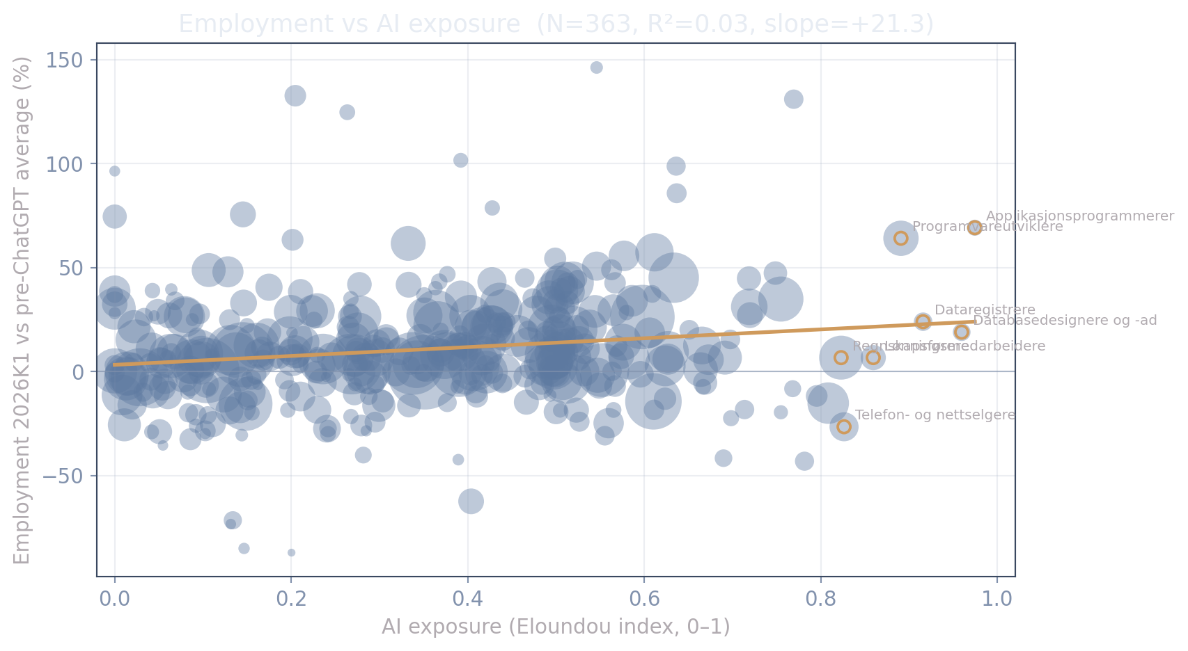
Employment growth against exposure
The cloud is flat-to-slightly-positive. Note two things, because they answer the obvious question “where are the 90–100%-exposure software jobs?”: the most-exposed occupations (programmers, database/data-entry, payroll) sit at exposure 0.86–0.97 (ringed) but employ only a few hundred to a few thousand each, so they barely move aggregate employment; and the single 100%-exposure occupation (“Kodere mv.”) is dropped, because SSB suppresses its wage (≈ 6–14 employed) so it has no wage to control for.
The regression: exposure, then control for wage, then the interaction
Effect on employment (percentage points), per 1 SD; robust SE in parentheses; *** p<.01, ** p<.05, * p<.1.
| Employment, % vs pre-ChatGPT avg (Yagan) | (1) exposure only | (2) + log pre-wage | (3) + interaction |
|---|---|---|---|
| AI exposure (β₁) | +4.4 (1.6)*** | +0.9 (1.9) | +1.5 (1.8) |
| log pre-ChatGPT wage (β₂) | +6.4 (1.8)*** | +5.9 (1.8)*** | |
| exposure × log wage (β₃) | +2.8 (2.0) | ||
| R² | 0.025 | 0.063 | 0.068 |
| N (occupations) | 357 | 357 | 357 |
Read it left to right — this is the whole story:
- (1) Naive. On its own, AI exposure looks good for jobs: +4.4 (1.6)***% per SD, significant. Exposed occupations grew. (The same lesson as the deck’s event-study exposure and comparative-advantage slides — both ≈ +3 pp.)
- (2) Control for pre-ChatGPT wage. The exposure coefficient collapses to +0.9 (1.9) — indistinguishable from zero — while the wage control takes a large, significant +6.4 (1.8)*. The naive “exposure effect” was wage in disguise**: high-exposure occupations are well paid, and well-paid occupations grew. OLS nets it out.
- (3) Add the interaction. Exposure stays at +1.5 (1.8) and the genuine interaction is +2.8 (2.0) — not significant. There is no extra job loss in high-wage exposed occupations: the sharp comparative-advantage prediction (\(\beta_3<0\)) does not show up.
The number that matters: total exposure effect by wage level
Because the effect of exposure now depends on wage, the quantity to report is the total exposure effect for an occupation, \(\beta_1+\beta_3\cdot(\text{wage})\):
| Total effect of +1 SD exposure | Employment |
|---|---|
| in a high-wage occupation (β₁ + β₃) | +4.3% [-1.7, +10.3] |
| in a low-wage occupation (β₁ − β₃) | -1.3% [-6.0, +3.4] |
Even at the top of the pay distribution — where displacement was predicted to bite hardest — the total employment effect of AI exposure is +4.3% [-1.7, +10.3], indistinguishable from zero. No displacement, including where the theory said to look for it.
The naive event study: exposure only
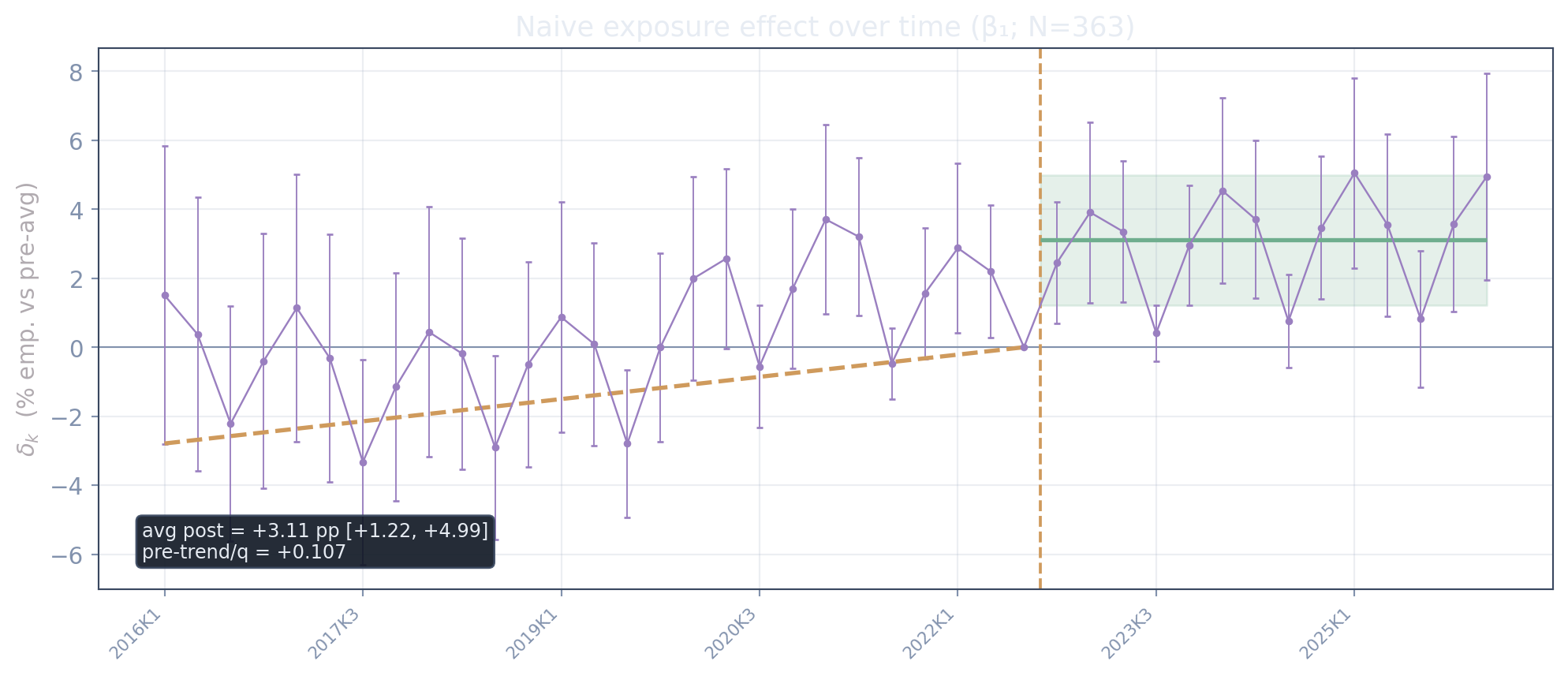
This is what people usually estimate — and on its own it looks like good news: +3.11 pp per SD post-ChatGPT. But the path shows a clear upward pre-trend (+0.107 pp/quarter) — exposed occupations were already drifting up before ChatGPT — which is exactly why the naive number cannot be read causally.
The same event study with heterogeneity by wage: the joint decomposition
The deck’s causal centerpiece. Exposure, the log wage, and their (centered) interaction each get a full set of quarter interactions, entered simultaneously — so the exposure path is net of wage, and the interaction path is the genuine does-exposure-bite-where-pay-is-high object (\(\beta_3 < 0\) is the displacement prediction).
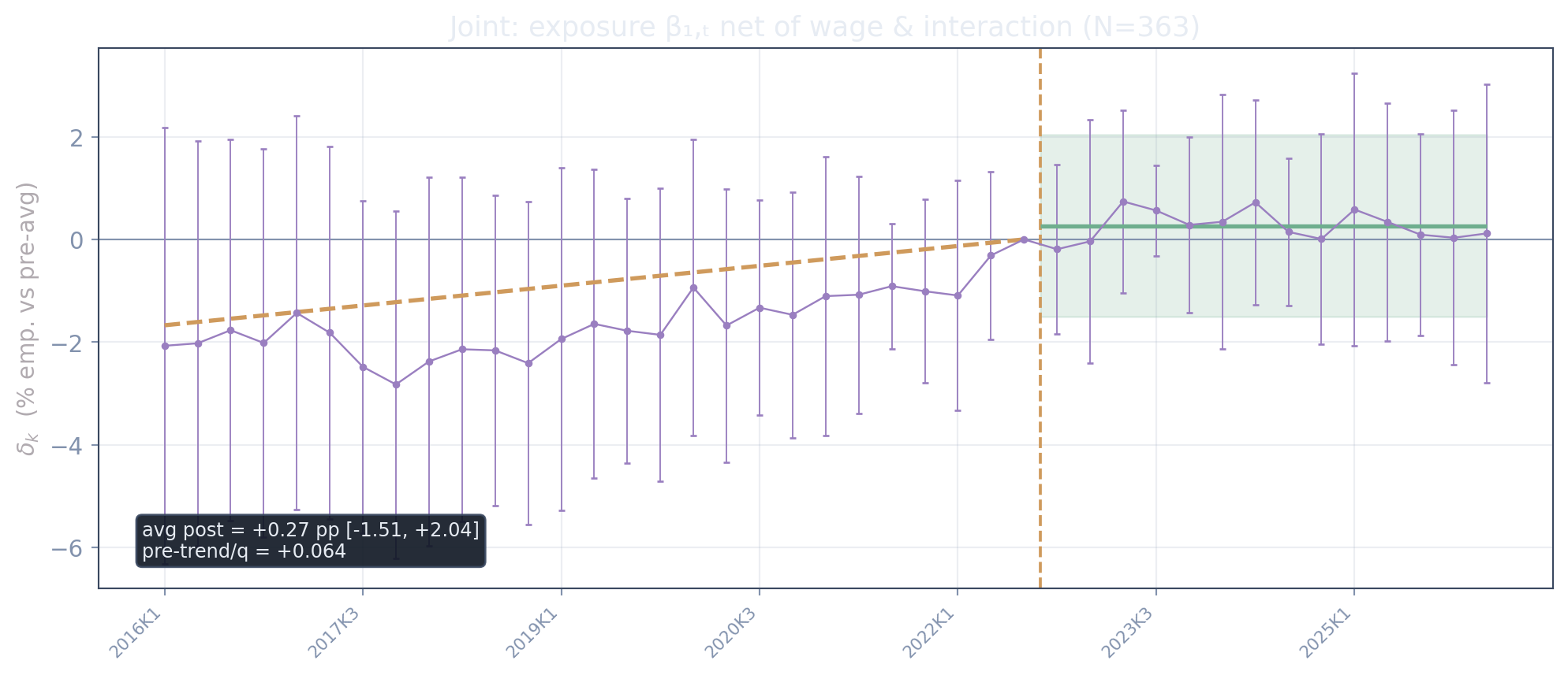
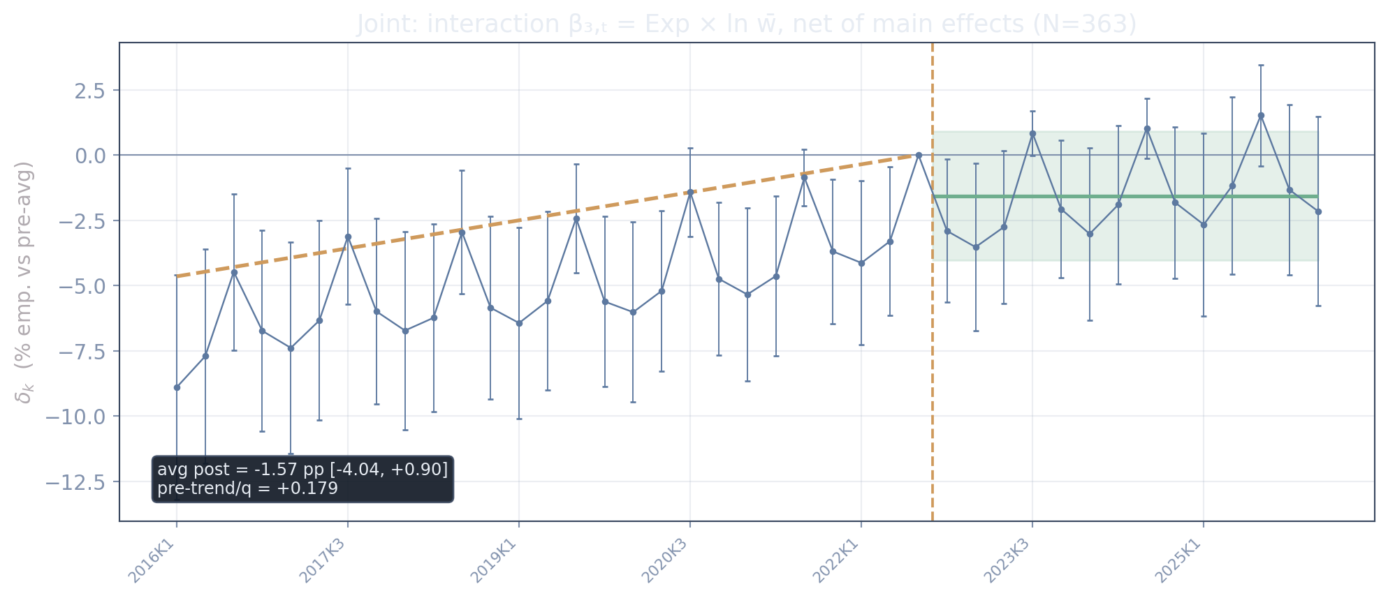
Net of the wage it travels with, exposure does nothing: the average post estimate is +0.3% [-1.5, +2.0]. And the interaction — the displacement object — is -1.6% [-4.0, +0.9], flat through the shock. The prediction \(\beta_3<0\) does not appear: even the well-paid, exposed occupations show no extra decline. (The comparative-advantage signal in a one-regressor fit is carried by the wage main effect, +4.8% [+1.7, +7.9].)
Causal interpretation: HonestDiD on naive vs joint
Per-SD average post effects with Rambachan–Roth (2023) relative-magnitudes robustness — the same table as the deck:
| avg post (pp/SD) | 95% CI | HonestDiD 95% CI (M̄=1) | breakdown M̄* | |
|---|---|---|---|---|
| Naive exposure only (β₁) | +3.11 | [+1.22, +4.99] | [-26.4, +32.6] | 0.04 |
| Joint fit: exposure (β₁) | +0.27 | [-1.51, +2.04] | [-8.4, +9.0] | n.s. |
| Joint fit: interaction (β₃) | -1.57 | [-4.04, +0.90] | [-32.4, +29.3] | n.s. |
- The only positive-looking estimate is the naive exposure effect (+3.1 pp/SD). Its breakdown is \(\bar M^\ast \approx 0.04\): a post-shock deviation from parallel trends just 4% as large as the worst pre-ChatGPT wobble already puts zero back in the interval — not robust.
- In the joint fit, exposure (β₁) and the genuine interaction (β₃) are already ≈ 0 — there is no positive effect left for a pre-trend to overturn.
- Causal verdict: no robust effect in either direction — no displacement, no dividend.
Bottom line
- The naive exposure effect is wage in disguise. +4.4 (1.6)**% per SD on its own → +0.9 (1.9)% once pre-ChatGPT wage is controlled; in the joint event study, exposure net of wage is +0.3% [-1.5, +2.0]. What grew were well-paid* occupations, exposed or not.
- No displacement, including where predicted. The heterogeneity-by-wage interaction is -1.6% [-4.0, +0.9] in the joint event study (+2.8 (2.0)% in the cross-section, n.s. both ways); the total exposure effect for a high-wage occupation is +4.3% [-1.7, +10.3] — zero. Aggregate employment in these 357 occupations rose 0.3% from 2022Q3 to 2026Q1 (2,767,939 employed in 2026Q1).
- And the naive positive effect is not robust either. A strong pre-trend drives it: HonestDiD breakdown \(\bar M^\ast \approx 0.04\). Causal verdict: no robust effect in either direction. Displacement, if it comes, should surface first in hiring and entry-level flows, which a stock panel understates — the next test.
Take this study into the AI Impact Analyst →
The analyst opens with every exhibit of this study loaded in the Exhibit picker, and can edit each one on request — change the specification, the standard errors, the wage definition, or the variables — and the revised figure or table appears directly in the chat.
References
- Lindenlaub, I., Oh, R., Rodríguez, M. A. & Veldkamp, L. (2026). Beyond Exposure: Predicting AI Adoption Based on Comparative Advantage.
- Eloundou, T., Manning, S., Mishkin, P. & Rock, D. (2024). GPTs are GPTs: Labor Market Impact Potential of LLMs.
- Rambachan, A. & Roth, J. (2023). A More Credible Approach to Parallel Trends. Review of Economic Studies.
- Statistics Norway (SSB), StatBank via PxWebApi v2 — tables 12542 (employment) and 11418 (monthly earnings).